Stereo Vision in OpenCV using your GPU

Stereo Visions algorithms, like Semi-Global Block Matching (SGBM), are quite slow. However it is possible to use the Graphics Processing Unit (GPU) of the computer to speed up algorithms to realtime speeds (30 FPS+).

OpenCV provides a whole range of Stereo Vision algorithms out of the box and from version 4.5.2 on it also provides SGM. Unfortunately installing OpenCV with CUDA/GPU support is not trivial. The easiest way to work with OpenCV and CUDA is to use a docker image from https://github.com/JulianAssmann/opencv-cuda-docker.

At the time of this post there was no OpenCV version 4.5.3 Docker Image on Dockerhub, so we take the Dockerfile here and we build it:

docker build -t opencv4.5.3 .

In order to easily call different algoritms we make a wrapper class:

import numpy as np
import cv2
from cv2 import cuda


class StereoWrapper:
    """
    This class takes care of the CUDA input such that such that images
    can be provided as numpy array
    """

    def __init__(self,
                 num_disparities: int = 128,
                 block_size: int = 25,
                 bp_ndisp: int = 64,
                 min_disparity: int = 16,
                 uniqueness_ratio: int = 5
                 ) -> None:
        self.stereo_bm_cuda = cuda.createStereoBM(numDisparities=num_disparities,
                                                  blockSize=block_size)
        self.stereo_bp_cuda = cuda.createStereoBeliefPropagation(ndisp=bp_ndisp)
        self.stereo_bcp_cuda = cuda.createStereoConstantSpaceBP(min_disparity)
        self.stereo_sgm_cuda = cuda.createStereoSGM(minDisparity=min_disparity,
                                                    numDisparities=num_disparities,
                                                    uniquenessRatio=uniqueness_ratio
                                                    )

    @staticmethod
    def __numpy_to_gpumat(np_image: np.ndarray) -> cv2.cuda_GpuMat:
        """
        This method converts the numpy image matrix to a matrix that
        can be used by opencv cuda.

        Args:
            np_image: the numpy image matrix

        Returns:
            The image as a cuda matrix

        """
        image_cuda = cv2.cuda_GpuMat()
        image_cuda.upload(cv2.cvtColor(np_image, cv2.COLOR_BGR2GRAY))
        return image_cuda

    def compute_disparity(self, left_img: np.ndarray,
                          right_img: np.ndarray,
                          algorithm_name: str = "stereo_sgm_cuda"
                          ) -> np.ndarray:
        """
        Computes the disparity map using the named algorithm.

        Args:
            left_img: the numpy image matrix for the left camera
            right_img: the numpy image matrix for the right camera
            algorithm_name: the algorithm to use for calculating the disparity map

        Returns:
            The disparity map
        """
        algorithm = getattr(self, algorithm_name)
        left_cuda = self.__numpy_to_gpumat(left_img)
        right_cuda = self.__numpy_to_gpumat(right_img)

        if algorithm_name == "stereo_sgm_cuda":
            disparity_sgm_cuda_2 = cv2.cuda_GpuMat()
            disparity_sgm_cuda_1 = algorithm.compute(left_cuda,
                                                     right_cuda,
                                                     disparity_sgm_cuda_2)
            return disparity_sgm_cuda_1.download()
        else:
            disparity_cuda = algorithm.compute(left_cuda, right_cuda, cv2.cuda_Stream.Null())
            return disparity_cuda.download()

Calling CUDA based algorithm in Python using OpenCV works a bit different than the OpenCV standard. This wrapper class helps you call it in a similar way:

left_img = cv2.imread("rectified_left.png")
right_img = cv2.imread("rectified_right.png")
wrapper = StereoWrapper()
disparity_map = wrapper.compute(left_img, right_img)
Data Augmentation with Keras

Training deep learning neural networks requires many examples to make the network better able to classify a new image. More examples can be created by data augmentation, i.e., change brightness, rotate or shear images to generate more data.

from keras.applications.inception_v3 import preprocess_input
from tensorflow.keras.preprocessing.image import ImageDataGenerator
from tensorflow.keras.models import Sequential
from tensorflow.keras.layers import Dropout, Flatten, Dense, GlobalAveragePooling2D
from tensorflow.keras import applications
from tensorflow.keras import regularizers
import tensorflow.python.keras.backend as K
from tensorflow.keras import optimizers, metrics

Import the ImageDataGenerator to do data augmentation with Keras. Furthermore get the preprocessing function preprocess_input to do the image preprocessing required by the deep learning architecture you use (Inception V3 in this example).

train_datagen = ImageDataGenerator(
    preprocessing_function=preprocess_input,
    brightness_range=[0.5, 1.2],
    shear_range=45.,
    rotation_range=90,
    validation_split=0.2)

Create one ImageDataGenerator that we will use for generating validation data and training data. Specifically we can see that the we make a 80% / 20% split. Furthermore we shear images upto a 45 degree angle; shearing is useful when you must classify images that are made at an angle.

train_generator = train_datagen.flow_from_directory(
    "D:\\train_examples_data",
    target_size=(img_height, img_width),
    batch_size=batch_size,
    class_mode='categorical', subset='training', shuffle=True)

nb_train_samples = train_generator.samples

The train_generator is set to flow / generate images from a directory on the Windows drive D. Furthermore this will generate the training subset (80%) and all images will be resized to the size required by the chosen deep learning architecture. Finally the number of images in the training data set is stored in the variable nb_train_samples.

In the same way we create a validation generator for generating validation data.

validation_generator = train_datagen.flow_from_directory(
    "D:\\train_examples_data",
    target_size=(img_height, img_width),
    batch_size=batch_size,
    class_mode='categorical', subset='validation', shuffle=True)

nb_validation_samples = validation_generator.samples

We will do transfer learning with Inception V3 where we first download the pretrained model.

model = applications.InceptionV3(weights='imagenet', include_top=False, input_shape = (img_width, img_height, 3))

Now a new top layer needs to be added and lower layer need to be set to be none trainable such that pre-trained weights aren’t lost. For the latter we make an extra function prepare_transfer. Set your own number of classes with the num_classes variable.

def prepare_transfer(model, reinit = True, keep_index = 229):
    session = K.get_session()
    for idx, layer in enumerate(model.layers):
        if idx < keep_index:
            layer.trainable = False
        elif reinit and hasattr(layer, 'kernel_initializer'):
            layer.kernel.initializer.run(session=session)
prepare_transfer(model, reinit = True, keep_index = 229)

top_model = Sequential()
top_model.add(GlobalAveragePooling2D(input_shape=(8, 8, 2048)))
top_model.add(Dense(num_classes, activation='softmax', kernel_regularizer=regularizers.l2(0.01), name='features', input_shape=(None, 2048)))

Add top and bottom layer together and compile the model.

new_model = Sequential()
new_model.add(model)
new_model.add(top_model)

new_model.compile(loss='categorical_crossentropy',
              optimizer=optimizers.RMSprop(lr=0.001),
              metrics=[metrics.categorical_accuracy])

Then we start training the model using the fit_generator function.

history = new_model.fit_generator(
    train_generator,
    steps_per_epoch=nb_train_samples/batch_size,
    epochs=epochs,
    validation_data=validation_generator,
    validation_steps=nb_validation_samples/batch_size,
    verbose = 1
)

Constructing a privacy plot using K-Means clustering

Nowadays the General Data Protection Regulation (GDPR) requires the data scientist to always guard the privacy of the people we study. For this reason this post will show how to make an extended scatterplot. That is we visualize, using clustering in R, only groups of people. As a result the groups that are visualized are of a minimum size as required by regulation and/or the organisation.

First of all install and load the required packages stats for k-means clustering and ggplot for visualization.

if(!(require(stats))) {install.packages("stats"); require(stats)}
if(!(require(ggplot2))) {install.packages("ggplot2"); require(ggplot2)}

Second of all construct a function for re-usability.

PrivacyPlot <- function(plot.data, xval, yval, min.points = 10, 
                        n.points = 5, decide.k = F, alpha=1.0, title = "") {
.....
}

Now we add the code to the function. First we cast to a matrix, because kmeans requires the data as a matrix. Secondly, we try different numbers of clusters k such that the number of clusters meeting the required number of points is largest.

data.matrix <- as.matrix(plot.data[,c(xval, yval)])
clustering <- kmeans(data.matrix, n.points)
if(decide.k) {
  for(k in 3:30) {
    clustering.k <- kmeans(data.matrix, k)
    if(sum(clustering.k$size >= min.points) > 
       sum(clustering$size >= min.points)) {
      clustering <- clustering.k
    }
  }
} 

Next select the centers of the clusters that meet the minimal size requirements. Furthermore make a data frame and normalize the size, because this is needed for ggplot to make a nice visualization.

  clustering.df <- as.data.frame(clustering$centers
  [clustering$size >= min.points,])
  clustering.df$cluster.size <- clustering$size
  [clustering$size >= min.points]
  clustering.df$cluster.size <- round(clustering.df$cluster.size * 30 / 
  max(clustering.df$cluster.size))

Finally visualize the results using ggplot and also include a trend line on the original data points.

  plt <- ggplot(clustering.df,
                aes_string(y=yval, x=xval)) +
    geom_point(shape=16, size=clustering.df$cluster.size, alpha=alpha) +
    geom_smooth(data = plot.data, method=lm) + ggtitle(title)
  
  return(plt)

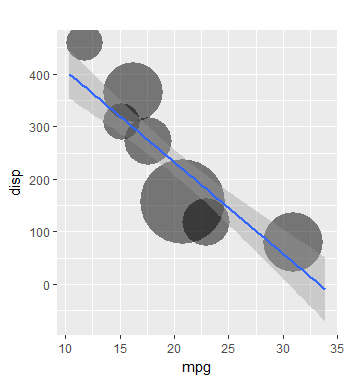
Additionally we can test our function using the mtcars dataset.

PrivacyPlot(mtcars, "mpg", "disp", min.points = 3, 
alpha = 0.5, decide.k = T)

So that this results in a scatterplot showing the trend and where the majority of points can be found. Also, in this example, the plot points represent a minimum of 3 points.

Privacy plot using k-means clustering.